Introduction

Chances are, if you’re going to do a mid-2000s to mid-2010s style sentiment analysis, you’re going to use a sentiment dictionary^{[These are also referred to as sentiment lexicons].}[Or, you might be a colleague of mine and publishing an article in PNAS in 2022. Congrats!] When reaching for one of these things, you’ve got quite a few options. This embarras de richesse should raise the question, Which should I use? I say “should raise the question” because I feel like all too often these dictionaries are presented as issue-free, ‘sure just go ahead and use it’ tools. For anyone who has studied measurement or thought about scale validation that is a truly apoplexy-inducing idea.

Both for your and my future reference, below I (will, upon completion) have a description of 10 or so dictionaries that I’ve come across quite a few times and found worth investigating why they were invented and if they should ever still be used.¹ Regardless of what I say below, remember that you’ll probably have to think about your application when choosing a dictionary; there is no one-size-fits-all best choice. Also, this post abstains from high-level thoughts about the entire enterprise of using sentiment dictionaries to get sentiment scores for sentences, utterances, documents, etc. That’s a different kettle of fish.²

With that, let’s go through these things in alphabetical order.

AFINN

The subtitle of the original publication says it all, “Evaluation of a word list for sentiment analysis in microblogs.” In the paper’s abstract, the great Dane and presumably the namesake of the lexicon, Finn Arup Nielsen, lays out more explicitly why he created a new sentiment lexicon, “There exist several affective word lists, e.g., ANEW (Affective Norms for English Words) developed before the advent of microblogging and sentiment analysis. I wanted to examine how well ANEW and other word lists performs for the detection of sentiment strength in microblog posts in comparison with a new word list specifically constructed for microblogs.” There’s AFINN’s origin story.³

One of the unique features of the AFINN lexicon is that words are mapped to integers instead of merely {positive, negative}. Here you can see a few words at each value:

set.seed(1)

get_sentiments('afinn') %>%
  group_by(value) %>% 
  add_count(name = 'count') %>% 
  slice_sample(n = 4) %>%
  summarise(
    `no. words` = mean(count),
    words = glue_collapse(word, sep = ', ')) %>% 
  arrange(value) %>% filter(value != 0)

# A tibble: 10 × 3
   value `no. words` words                                      
   <dbl>       <dbl> <glue>                                     
 1    -5          16 motherfucker, bitches, cocksuckers, bastard
 2    -4          43 scumbag, fucking, fraudsters, fucked       
 3    -3         264 moron, destroy, despair, scandals          
 4    -2         966 animosity, censors, robs, touts            
 5    -1         309 imposing, unclear, demonstration, uncertain
 6     1         208 share, extend, feeling, commit             
 7     2         448 tranquil, consent, supportive, sympathetic 
 8     3         172 audacious, classy, luck, gracious          
 9     4          45 exuberant, wonderful, rejoicing, wowww     
10     5           5 hurrah, outstanding, superb, thrilled

And yes, I did set the seed above to avoid randomly showing you certain words.

You might be wondering

why -5 to 5 and
how he assigned words to those numbers

Quoting him on the former, “As SentiStrength it uses a scoring range from −5 (very negative) to +5 (very positive).” Convention is powerful. As for the latter, the question of how numbers were assigned to words, “Most of the positive words were labeled with +2 and most of the negative words with –2 […]. I typically rated strong obscene words […] with either –4 or –5.” So he was basically winging it.

Another unique feature: the dictionary has 15 bigrams, 10 of which are below.⁴

set.seed(12)
get_sentiments('afinn') %>%
  filter(str_detect(word, ' ')) %>% 
  slice_sample(n = 10)

# A tibble: 10 × 2
   word          value
   <chr>         <dbl>
 1 cashing in       -2
 2 no fun           -3
 3 green wash       -3
 4 not good         -2
 5 dont like        -2
 6 not working      -3
 7 some kind         0
 8 green washing    -3
 9 cool stuff        3
10 messing up       -2

Size: 2477 entries
Coverage: In addition to the bog-standard sentiment words, it has words all the cool kids were saying in the late 2000, early 2010s.
R Packages: tidytext, lexicon, textdata
Publication: Here
Bottom Line: It’s been superseded by VADER (below)

Bing (aka Hu and Liu)⁵

According to the man himself, “This list [i.e., the lexicon] was compiled over many years starting from our first paper (Hu and Liu, KDD-2004).” I’m not sure what the post-publication compilation process was, but the original process is well-described in the original publication. Essentially, they started with adjectives⁶ with obvious polarity (e.g., great, fantastic, nice, cool, bad, dull) as ‘seed words’ and collected synonyms (and antonyms) of those words, then synonyms and antonyms of those words, and so on, iteratively. To do this, they used WordNet, a chill-ass semantic network. One thing that’s nice about the resulting lexicon is that it’s topic general. That is, though they developed this lexicon for the specific purpose of determining people’s opinions about product features in product reviews, it has a generality beyond that.

Actually looking at the words, you’ll notice there’s some weirdness.

head(get_sentiments('bing'), 10)

# A tibble: 10 × 2
   word        sentiment
   <chr>       <chr>    
 1 2-faces     negative 
 2 abnormal    negative 
 3 abolish     negative 
 4 abominable  negative 
 5 abominably  negative 
 6 abominate   negative 
 7 abomination negative 
 8 abort       negative 
 9 aborted     negative 
10 aborts      negative

First, I’m not sure what “2-faces” is. If you say that it’s a solecistic rendering of “two-faced,” I’d say probably. In their appropriate alphabetic order, both “two-faced” and “two-faces” appear later in the dictionary. Anyway, you’ll notice as well that a lot of the words would reduce to a single lemma if we lemmatized the dictionary. You can think of that as a positive feature of the BING dictionary. It means you don’t have to have lemmatized (or stemmed) text. But its inclusion of derived words seems a bit haphazard. The abort-aborted pair is there, but abolish is hanging out along without its past tense.

Size: In the tidytext package the BING dictionary has 6786 terms (matching what his website says, “around 6800 words”)
R Packages: tidytext, lexicon, textdata
Bottom Line: It’s a classic and got wide coverage, but not as good as VADER or NRC-EIL.

Loughran-McDonald Master Dictionary w/ Sentiment Word Lists

I’m honestly why this dictionary is included in packages – not because it’s bad⁷, but because it’s so (so so so) niche. If you’re doing text analysis on financial text (or aware of cool research doing this), please drop me a line and tell me about it.

If you want to learn about it, here’s the page.

R Packages: tidytext, lexicon, textdata

NRC (original)

Saif Mohammad and friends developed a few National Research Council (NRC) of Canada-sponsored sentiment dictionaries. The first of them assigns words not only polarity labels (positive, negative), but emotion labels as well:

tidytext::get_sentiments('nrc') %>% 
  count(sentiment, sort = TRUE)

# A tibble: 10 × 2
   sentiment        n
   <chr>        <int>
 1 negative      3318
 2 positive      2308
 3 fear          1474
 4 anger         1246
 5 trust         1230
 6 sadness       1187
 7 disgust       1056
 8 anticipation   837
 9 joy            687
10 surprise       532

These eight emotions below negative and positive were theorized by Bob Plutchik to be fundamental, or something.⁸ I’m going to ignore those emotions in this subsection. I’m also not going to talk too much about this dictionary, because it’s superseded by the real-valued its successors, the NRC-EIL and NRC-VAD (below).

Before I leave this lexicon, though, one bizarre thing about it: 81 words are both positive and negative (???)

get_sentiments('nrc') %>% 
  filter(sentiment %in% c('negative', 'positive')) %>% 
  add_count(word) %>% 
  filter(n > 1) %>% select(-n)

# A tibble: 162 × 2
   word       sentiment
   <chr>      <chr>    
 1 abundance  negative 
 2 abundance  positive 
 3 armed      negative 
 4 armed      positive 
 5 balm       negative 
 6 balm       positive 
 7 boast      negative 
 8 boast      positive 
 9 boisterous negative 
10 boisterous positive 
# ℹ 152 more rows

As a matter of semantics, I get it for some of these (balm I do not get, though). Practically, if you’re doing an analysis with this dictionary, you’re probably going to want to remove all these terms before calculating sentiment scores.

R Packages: tidytext, lexicon, textdata
Size: 5464 words (positive and negative, not words with ambiguous polarity)
Bottom Line: Superseded by Saif Mohammed’s subsequent efforts.

NRC-EIL

This thing’s value-added, as my economist friend likes to say, is that instead of a simple ‘positive’ or ‘negative’ value for each sentiment entry, there’s a number between -1 and 1. “Real-valued,” as measurement-heads say. This is actually extremely important if you’re aggregating word-level sentiment into something bigger (which … honestly, email me if you’re doing anything other than that.) How they got these real-valued polarity scores is actually a pretty interesting methods story if you’re into that kind of thing, but I won’t go into ‘MaxDiff scaling’ here. One very important thing to note about this dataset, though, is that valence is that polarity isn’t in this dataset. This vexed me for a minute before I realized that it’s in the real-valued NRC-VAD (below). So, on the off chance you’re looking for the best measurement of Plutchik’s eight basic emotions (and that’s a very off chance), this is the best place to look.

R Packages: textdata
Examples: You can see an example of an analysis of Ezra Klein’s podcasts here.
Bottom Line: I’m not sure why it exists, but it’s the only lexicon doing what it’s doing.

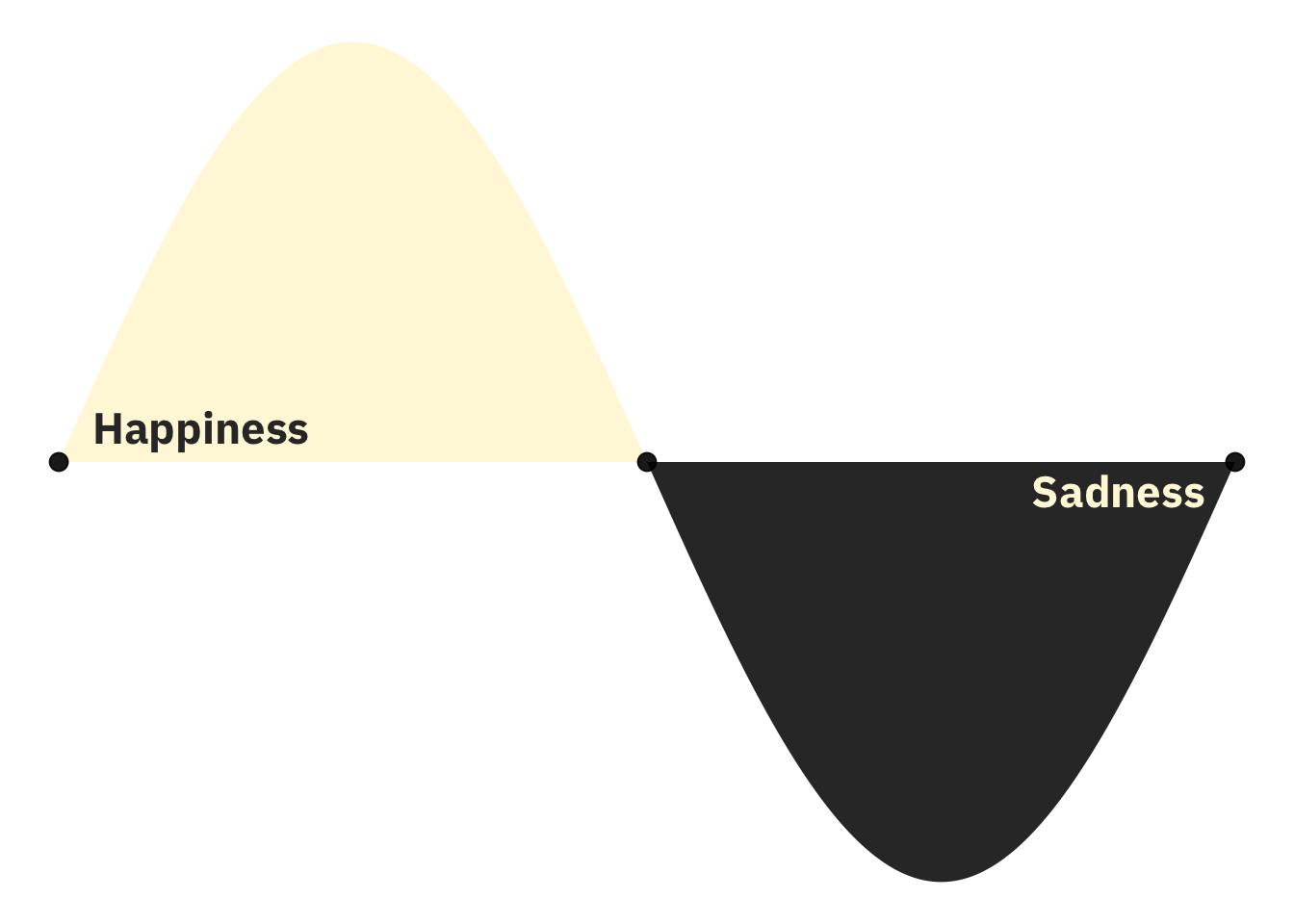
NRC-VAD

Once you have a hammer, everything starts looking like a nail. That’s how I explain the existence of this dictionary to myself. Saif Mohammed & Co. found these cool scaling technique and were like, “On what dimensions can we scale more words?” They seem to have stumbled on this idea the three most fundamental dimensions in concept space are valence, arousal, and dominance. Maybe it’s an indictment of my memory, perhaps an indictment of the psychology department at the University of Arkansas, but I managed to graduate summa cum laude with a degree in psychology without ever hearing of this. Regardless of supposed fundamental dimensions in concept space, valence is fundamental and is just another word for polarity which is the main thing people are doing with sentiment dictionaries.

This also led to my favorite table in I’ve ever seen in an academic article

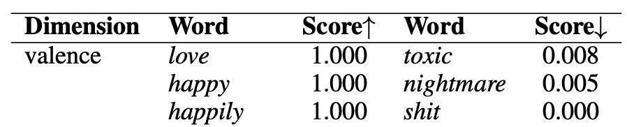
Whenever I need to express that something is pure bad valence, I now reach for the phrase ‘toxic nightmare shit.’

R Packages: textdata
Bottom Line: Hell yeah. This is a good one.

SOCAL

It’s the Semantic Orientation CALculator! Like VADER (below), SOCAL is both a sentiment dictionary and rules for modifying words’ sentiment given the context in which they appear. Below, I’ll only briefly consider the dictionary part. I recommend reading the publication both for more details on SOCAL itself as well as sentiment analysis generally. In a sea of sentiment articles that are slapdash publications from some “Proceedings of blah blah blah” or “Miniconference on yak yak yak” this one really stands out for its professionalism and thoroughness.⁹ As for whether or not you should actually use this dictionary, uh, you should keep reading.

One fun thing to note about SOCAL’s dictionary: it has more entries with spaces than any other dictionary I’ve seen.

hash_sentiment_socal_google %>% 
  group_by(n_gram = str_count(x, ' ') + 1) %>% 
  count(n_gram) %>% 
  ungroup()

# A tibble: 8 × 2
  n_gram     n
   <dbl> <int>
1      1  2071
2      2  1097
3      3    97
4      4    17
5      5     3
6      6     3
7      7     1
8      8     1

This dictionary has not only a huge bigrams:unigrams ratio, but it has sextagrams, a septagram, and even an octogram! This never happens! Let’s look at the n-grams where n > 4

hash_sentiment_socal_google %>% 
  filter(str_count(x, ' ') > 3)

Key: <x>
                                                           x         y
                                                      <char>     <num>
1:                          darker and funnier than expected -4.092375
2:                                     every other word is f -1.955614
3:                          in your face everywhere you turn -5.357512
4: lowbump bump bump bump bump bump bumpbumpbumpbump lowbump  5.622471
5:                     throw your peanut shells on the floor -5.186874
6:                                      trying to get on top -2.573428
7:                               type stype suh huh uh huh's -4.281949
8:                            write an awesome story to sell -6.262021

I, uh, don’t really know what to make of these. There’s actually a restaurant named “Lambert’s Cafe” in Ozark, Missouri where you get peanuts in tin buckets and “throw your peanut shells on the floor” and, unless I’m remembering it wrong, it’s something people like about the place.

Speaking of things that are starting to be concerning, the distribution of scores:

library(ggtext)
ggplot(hash_sentiment_socal_google, aes(y)) +
  geom_density() +
  labs(
    y = '',
    x = 'Valence Score',
    title = '**What tale tell ye**, ye two thick tails?'
  ) +
  theme(plot.title = element_markdown(face = 'italic'))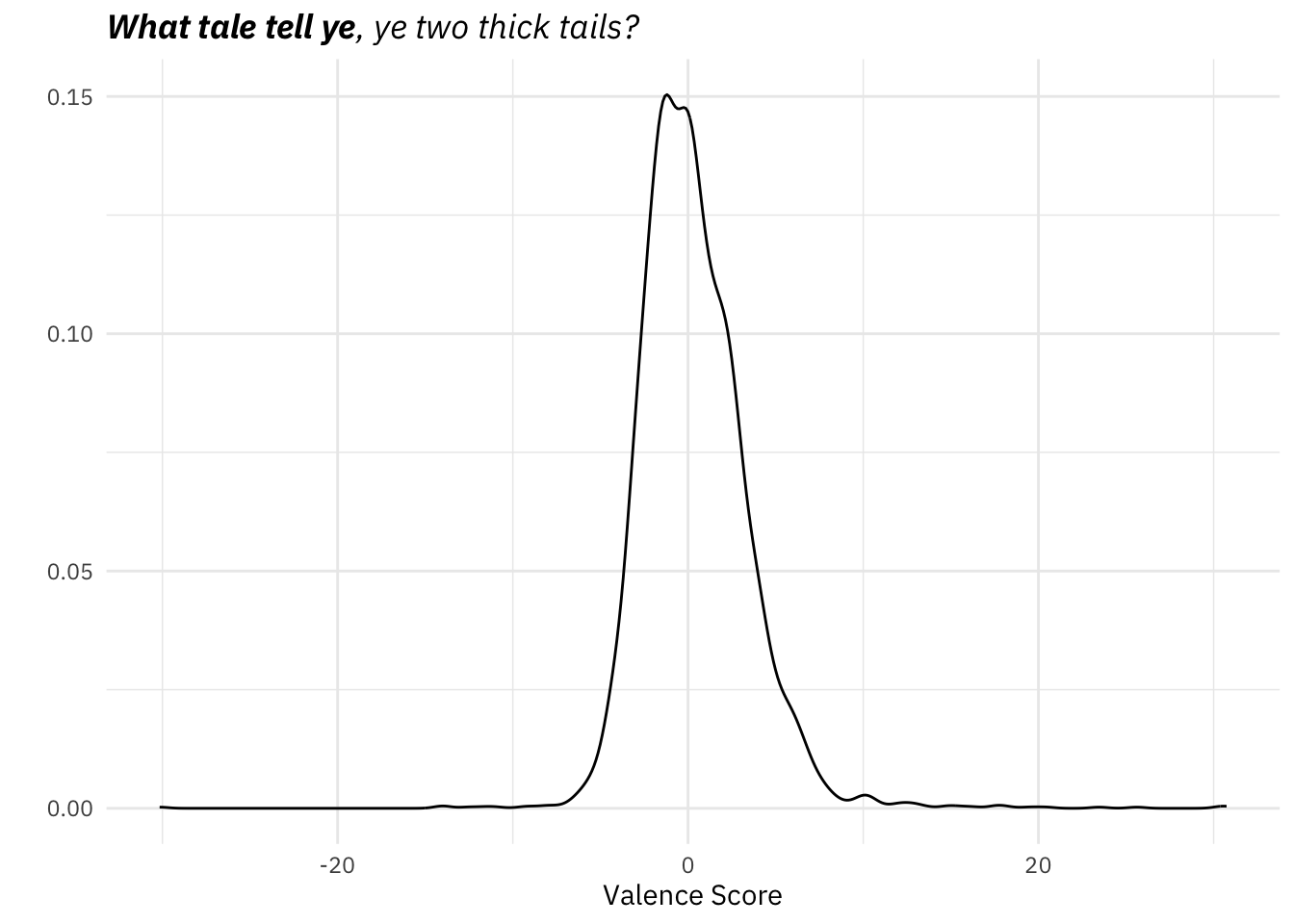

No, that density plot isn’t glitching. There really are words out there in the extremes:

hash_sentiment_socal_google %>% 
  filter(abs(y) > 15)

Key: <x>
                            x         y
                       <char>     <num>
 1:    almost mafiosio styled  15.61625
 2: automatically bestselling  17.60440
 3:        coming of age isms  17.62518
 4:           cushion handled  23.45929
 5:                 hop ified -30.16008
 6:          keyboard crafted  30.73891
 7:      more than palateable  25.61696
 8:          oven to stovetop  19.49040
 9:             piano blessed  30.40257
10:   rustic yet contemporary  16.31055
11:           slotted spooned  18.19201
12:              thick spoked  20.43281

At this point, you might be wondering … what scale is this? And what are values for our vanilla valence-indicators “good” and “bad”?

hash_sentiment_socal_google %>% 
  filter(x %in% c('good', 'bad'))

Key: <x>
        x         y
   <char>     <num>
1:    bad -1.636520
2:   good  1.872093

Ok, that’s fine. Maybe. But here’s something that probably isn’t fine:

hash_sentiment_socal_google %>% 
  filter(str_detect(x, 'good|bad'))

Key: <x>
                  x          y
             <char>      <num>
1:     average good  0.4205258
2:              bad -1.6365198
3:        feel good  1.2984294
4:             good  1.8720931
5: good intentioned -4.1537399
6:     good natured -1.5298719
7:         half bad -3.9237520

Here is where I lost all faith. “Good intentioned” and “good natured” are negative?!

At this point I’m going to call it a day with SOCAL. At some point I might write to the SOCAL authors or Tyler Rinker to see if something has gone wrong.

Publication: Again, I truly recommend it
Size: 3290 entries
R Packages: lexicon

Syuzhet

“The default method,”syuzhet” is a custom sentiment dictionary developed in the Nebraska Literary Lab. The default dictionary should be better tuned to fiction as the terms were extracted from a collection of 165,000 human coded sentences taken from a small corpus of contemporary novels.”

Now, it does include a lot of words I find to be neutral (e.g., “yes”, “true”)

We can check out the distribution of the terms in my experimental sideways histogram below:

# ggplot(key_sentiment_jockers, aes(value)) +
#   geom_histogram(breaks = seq(-1, 1, by = 0.1), color = 'white') +
#   theme(
#     panel.grid.major.x = element_blank(),
#     panel.grid.minor.x = element_blank(),
#     axis.text.x = element_text(margin = margin(t = -10, b = 5)),
#     plot.title = element_text(face = 'bold', size = rel(1.3))) +
#   scale_y_continuous(breaks = c(500, 1000, 1500)) +
#   labs(
#     x = 'Jockers/Syuzhet Value',
#     y = 'Terms in Dictionary',
#     title = 'Distribution of Sentiment Values in Syuzhet Dictionary'
#   )

distinct_values <- pull(distinct(key_sentiment_jockers, value))

ggplot(key_sentiment_jockers, aes(value)) +
  geom_bar(width = .07, alpha = 0.8, fill = c(viridis::magma(8, direction = -1), viridis::mako(8))) +
  geom_text(stat = 'count', aes(label = after_stat(count)), 
            hjust = -0.1,
            position = position_stack(),
            family = 'IBM Plex Sans',
            face = 'bold') +
  scale_x_continuous(breaks = distinct_values) +
  theme(
    panel.grid.major.y = element_blank(),
    panel.grid.minor.y = element_blank(),
    plot.title = element_text(face = 'bold'),
    axis.text.y = element_text(margin = margin(r = -20))) +
  coord_flip() +
  labs(x = 'Valence Value in Syuzhet',
       y = 'Counts',
       title = 'Distribution of Sentiment Values in Syuzhet Dictionary') +
  geom_vline(xintercept = 0)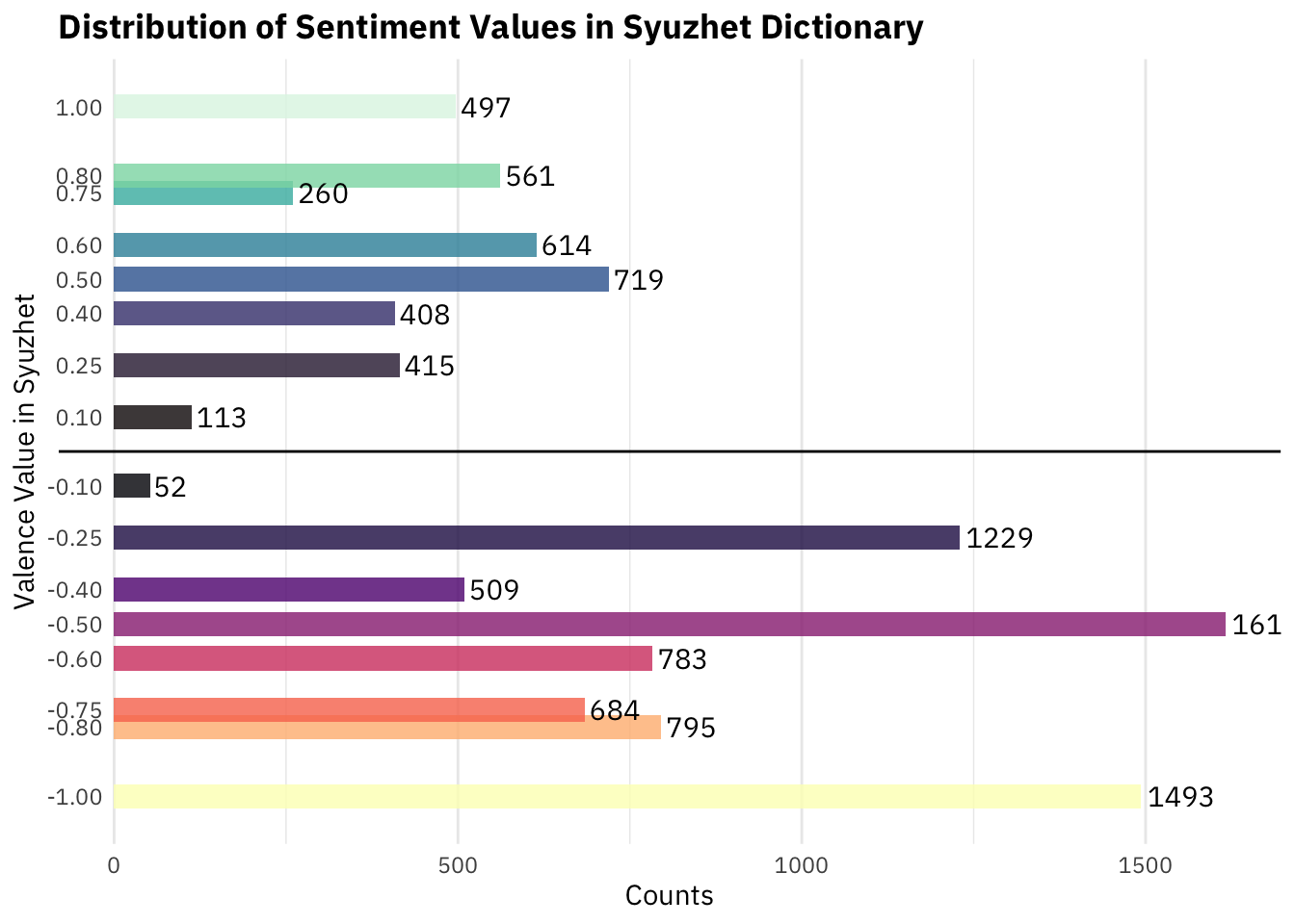

R Packages: syuzhet, lexicon
Size: 10,748 words
Bottom Line: Pending.

VADER

Is VADER evil? Maybe. But it also stands for Valence Aware Dictionary and sEntiment Reasoner.¹⁰ Impressively, the found “that VADER outperforms individual human raters” when classifying tweets as positive, accurate, or neutral.¹¹ Part (most?) of that impressiveness is due to the ‘ER’ of VADER. Nevertheless, here I’m only considering the VAD part. If you want to check out its ruled-based sentiment reasoning, check out its github page or publication.

The lexicon has an impressive 7,500 entries, each with its associated polarity and intensity (-4 to 4). Did they get those intensities just winging it like Finn? Nope. Each potential entry was placed on the -4 to 4 scale by 10 Amazon Mechanical Turk workers.¹² The score you do see in the dictionary means that a) raters’ scores had a standard deviation of less than 2.5¹³ and b) that the mean rating among the 10 raters was not 0.¹⁴

One interesting feature of the lexicon is its inclusion of emoticons.

vader <- read_delim('https://raw.githubusercontent.com/cjhutto/vaderSentiment/master/vaderSentiment/vader_lexicon.txt',
                    delim = '\t', col_names = FALSE) %>% magrittr::set_names(c('token', 'score', 'sd', 'scores'))

vader %>% 
  filter(str_detect(token, '[A-Za-z1-9]', negate = TRUE)) %>% 
  group_by(bin = score %/% 1) %>% 
  mutate(y = row_number()) %>% 
  ungroup() %>% 
  ggplot(aes(bin, y, label = token)) +
  geom_text(check_overlap = TRUE, fontface = 'bold', family = 'IBM Plex Sans') +
  scale_y_continuous(NULL, breaks = NULL) +
  labs(
    x = '',
    caption = 'To reduce the real-valued chaos, I rounded down emoticons\' scores to the nearest integer'
  ) +
  theme(
    panel.grid.major.x = element_blank(),
    axis.text = element_text(face = 'bold'),
    panel.grid.minor.x = element_line(linetype = 2, color = 'grey35')
  ) +
  guides(color = 'none')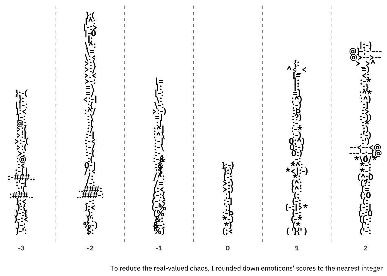

I don’t want to make this dictionary seem trivial. Its creators also validated it using sentences from New York Times editorials, as well. It’s just not every day that you can make a histogram of emoticons.

R Packages: As far as I know, it’s not in any. You can get it directly from its github repository.
Side Benefit: This is probably the one that your “pythonista” friends are familiar with, since it’s in the nltk library.

Coverage Comparison for AFINN, BING, and NRC

afinn <- get_sentiments(lexicon = 'afinn')
bing <- get_sentiments(lexicon = 'bing')
nrc_emotions <- filter(get_sentiments(lexicon = 'nrc'), 
                    !(sentiment %in% c('positive', 'negative')))
nrc_polar <- filter(get_sentiments(lexicon = 'nrc'), 
                    sentiment %in% c('positive', 'negative'))

bind_rows(
  select(mutate(afinn, lexicon = 'AFINN'), word, lexicon),
  select(mutate(bing, lexicon = 'BING'), word, lexicon),
  select(mutate(nrc_polar, lexicon = 'NRC'), word, lexicon)) %>% 
  summarise(Lexica = list(lexicon), .by = word) %>% 
  ggplot(aes(Lexica)) +
  geom_bar() +
  scale_x_upset(n_intersections = 7) +
  theme_minimal() +
  theme(
    panel.grid.major.x = element_blank(),
    panel.grid.minor.y = element_blank(),
    title = element_text(family = "IBM Plex Sans"),
    plot.title = element_text(face = 'bold'),
    plot.subtitle = element_markdown(),
    axis.text = element_text(family = "IBM Plex Sans")
  ) +
  labs(
    y = 'Set Size',
    x = 'Set',
    title = 'Are Bigger Dictionaries Mostly Supersets of Smaller Dictionaries?',
    subtitle = "*No*, and that's weird"
  )

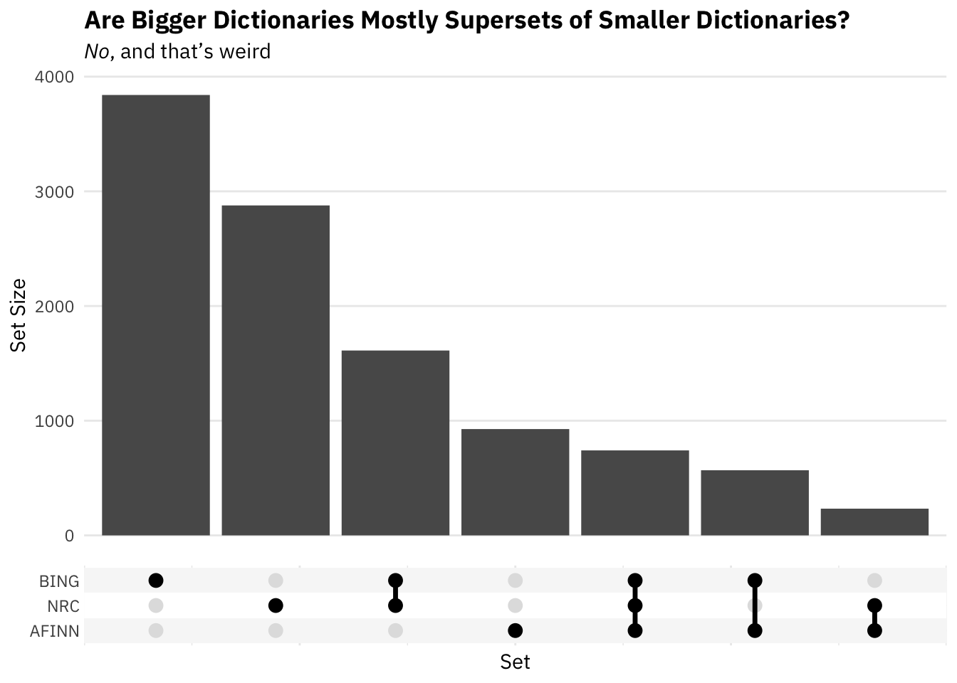
We can see how many entries each dictionary has:

c(nrow(afinn), nrow(bing), nrow(nrc_polar))

[1] 2477 6786 5626

Here we see a surprising amount of non-overlap. Of Bing’s 6786 terms, almost 4,000 do not appear in either of the other two dictionaries. Almost 3,000 of NRC’s polarity entries aren’t in either of the other two, as well. The third bar indicates that BING and NRC share just over 1,500 words. The short and long of this is that it might be important which dictionary we choose. They have very different coverages.¹⁵

Still to do

This page, like the rest of my life, is a work in progress.

I still have a few dictionaries to add. In Tyler Rinker’s lexicon package there are: jockers (and jockers_rinker), emojis (and emojis_sentiment), senticnet, sentiword, slangsd. I’ve already covered all dictionaries in tidytext and textdata.
Further comparison of dictionary overlap. 2a. Right now I look at three dictionaries’ overlap. These three aren’t the best, they’re just the first ones I checked out. That’s not a principled criterion for selecting dictionaries. I’ll redo that section programmatically. 2b. I’m going to lemmatize/stem the dictionaries covered and get their size and overlaps as I did with AFINN, BING, and NRC above. It’s possible that sizes are much more similar once you remove a bunch of morphological tangle.
Inspired by this sentence from Nielsen, “The word list have a bias towards negative words (1598, corresponding to 65%) compared to positive words (878)” I’m also going to see what the respective positive/negative balances are of these dictionaries.

Notes on Sentiment Dictionaries

Introduction

AFINN

Bing (aka Hu and Liu)⁵

Loughran-McDonald Master Dictionary w/ Sentiment Word Lists

NRC (original)

NRC-EIL

NRC-VAD

SOCAL

Syuzhet

VADER

Coverage Comparison for AFINN, BING, and NRC

Still to do

Recommended Usage and Tendentious Postscript

Footnotes

Introduction

AFINN

Bing (aka Hu and Liu)5

Loughran-McDonald Master Dictionary w/ Sentiment Word Lists

NRC (original)

NRC-EIL

NRC-VAD

SOCAL

Syuzhet

VADER

Coverage Comparison for AFINN, BING, and NRC

Still to do

Recommended Usage and Tendentious Postscript

Footnotes

Bing (aka Hu and Liu)⁵